Clustering is one of the fundamental tasks in unsupervised learning, but there are a huge diversity of approaches. There is k-means , mean-shift, hierarchical clustering, mixture models and more. The reason for so many varied approaches is that clustering by itself is ill-defined. In this post I will focus on two methods, mean-shift and Gaussian mixture modeling, because they have a more “statistical” flavor, in that they can be related to modeling a probability distribution over the data. Despite their similarities, they are based on sometimes contradictory principles.
1. Mean-shift
Mean-shift clusters points by the modes of a nonparametric kernel density. The kernel density estimator for data \(x_1,\ldots,x_N\) is
\(\hat{p}(x) =\frac{1}{nh^d} \sum_{i=1}^NK(\frac{\Vert x-x_i\Vert^2}{h}),\)
where \(K\) is a kernel function. You can imagine the kernel to be some density with variance one, such as a Gaussian density, with variability controlled by the bandwidth \(h\). In effect a kernel density is a smoothed histogram, a mixture of local densities at each datum. \(\hat{p}\) has some number of modes, let’s say \(p \).
The gradient of the density at a point \(x\) looks like
\( \nabla \hat{p}(x) = L(x)\cdot\left( \frac{ \sum_{i=1}^N x_i k(\frac{\Vert x-x_i\Vert^2}{h})}{\sum_{i=1}^n k(\frac{\Vert x-x_i\Vert^2}{h})} - x \right), \)
where \(L(x)\) is a positive function, \(k=K’\) and the second term is called the mean-shift, which we denote \(m(x)\). Any mode of \(\hat{p}\) will satisfy the fixed point \(m(x)=0\).
Mean-shift works as follows. Initialize \(w_1\) at some point. Then iterate the following until convergence:
\(w_t \leftarrow w_{t-1} + m(w_{t-1}).\)
Each iteration moves the point in an ascent direction of the density. Eventually it will converge to a fixed point, which is one of the modes of \(\hat{p}\). We do this for each data point, and we assign clusters based on which fixed point it converged to.
It’s well known that the kernel density is a consistent estimate of the true density for large sample size (and further, it’s modes are consistent as well). But there’s not a lot of understanding on guarantees for mean-shift itself. Also, density estimation is sensitive to bandwidth, and the number of modes can change for different choices of \(h\).
2. Mixture Models
Mixture models cluster based on a most probable assignment to a mixture component. It provides a generative interpretation for the data. It can do “soft clustering”, which means it provides not just the most probable cluster assignment, but the full probability vector (known as the responsibilities) for a datum belonging to all the clusters. In addition to clustering you also get a predictive density at no extra cost.
We may think of a Gaussian mixture model as a latent variable model. Suppose we have a random vector \(Y \sim Multinomial(1,p)\), that is \(Y\) chooses one value of \(\{1,\ldots,D\}\) according to probabilities \(p_1,\ldots,p_D\). Furthermore, for \(j\in \{1,\ldots,D\}\), we suppose \(Z_j \sim Normal(\mu_j,\Sigma_j)\), with each \(Z\) mutually independent and independent of \(Y\). A random vector \(X\) is a Gaussian mixture when we write it as.
\( X = \sum_{j=1}^D Y_j Z_j .\)
The density for a D-component GMM is given by
\(p(x \mid \{\theta_j, \mu_j,\Sigma_j\}_{j=1}^D ) = \sum_{j=1}^D \theta_j N(x \mid \mu_j,\Sigma_j), \)
where \(N(x \mid \mu,\Sigma)\) is a normal density. We maximize the log-likelihood:
\( \max_{\left\{\{\theta_j, \mu_j,\Sigma_j\}_{j=1}^D\right\}} \sum_{i=1}^N \log p(x \mid \theta, \{\mu_j,\Sigma_j\}_{j=1}^D ) . \)
This can be treated as a standard smooth optimization and use any solver of choice, but it’s more common to use the EM-algorithm.
The optimization of a GMM has some peculiar characteristics. Firstly, the likelihood has singularities. Suppose one of the clusters has a mean equal to one of the data. As the variance of the cluster goes to zero (so that one of the clusters becomes a point mass at the datum), the overall likelihood becomes unbounded. In such cases we say the maximum likelihood does not exist, but in practice we can often get a good solution which corresponds to some local optimum if we start at a reasonable initialization. Another phenomenon with mixture models is the “label switching” problem: there are always D! equivalent solutions corresponding to permutations of the parameter values among the clusters.
For a Gaussian mixture model, the number of modes of the density may be more or less than the number of clusters [1]. Also, the modes will generally not agree with the component means. Mixture modeling and mean-shift are really solutions to two different clustering objectives.
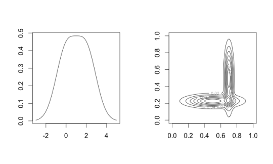
Figure 1: Left: a two-component mixture with one mode; Right: a two-component mixture with three modes.
We still have the issue of selecting the number of clusters. This is similar to choosing the bandwidth in mean-shift. Increasing D will always increase the log-likelihood objective, so you must select using a penalized score like BIC. However, BIC is designed to find a “good” model in the sense of density estimation. This is not necessarily the same as a “good” clustering, which we explained earlier is not well defined.
There are several good implementations of GMM, such as mclust in R. There is also an implementation for distributed data in Apache Spark MLLIB.
3. Demo
To demonstrate I fit the Gaussian mixture model in mclust to the faithful data set, a classic set of measurements of eruption/waiting time pairs at Old Faithful. mclust compares various types of models (spherical, elliptical, equal or different variances, etc.). Here BIC chooses 3 ellipsoidal Gaussian components. Two components are close together, resulting in many points having a high degree of classification uncertainty.
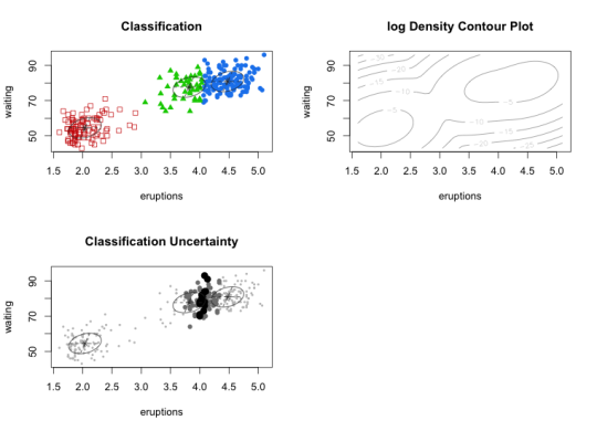
Figure 2: GMM Clustering on faithful data set
Next I try mean-shift using the R package LCPM. Using the bandwidth chosen by something called “self-coverage”. We see the algorithm converges to two modes.
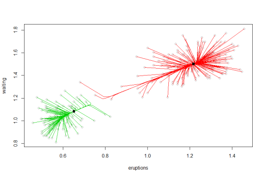
Figure 3: Mean-shift gradient curves for faithful data set.
Both of these methods give results that look a little funny. It may be surprising that GMM chose three clusters instead of two. Mean-shift chooses two clusters, but a few of the cluster assignments look surprising. One interesting property of mean-shift is a data point need not be assigned to the closest cluster center (according to some distance), because a mode may have a very large basin of attraction in the density. The cluster center is also not the literal “center” of the data in that cluster. GMM has three clusters but with a lot of classification uncertainty between two of them, while mean-shift classifies some points to the larger cluster which GMM assigned very little uncertainty of being in the smaller cluster! Also observe that the GMM density, despite having three mixture components, only has two modes. We should appreciate that these methods are really approaching clustering with two possibly incompatible philosophies.
I hope this shows the challenges in clustering even for the simplest of datasets.
There are some Bayesian treatments of Gaussian mixtures that I really like, which overcome several of the limitations of the aforementioned approach. I am working on a project to implement them in Spark. I will do a separate post on the details