The moments of a random variable \(X\) are given by \(\mathbb{E}[X^n]\), for all integers \(n\geq 1\). One fascinating fact I first learned while studying distribution theory is that the moment sequence does not always uniquely determine a distribution.

Consider \(X\sim logNormal(0,1)\), that is, \(log(X)\) follows a standard normal distribution, and let the density of \(X\) be \(f(x)\). The moments of \(X\) exist and have the closed form

\[ m_i := \mathbb{E}[X^i] = e^{i^2/2}. \]

Consider the density

\[ f_a(x) = f(x)(1+\sin(2\pi\log(x))), \,\,\, x\geq 0. \]

Then \(f,f_a\) have the same moments. To prove this, it’s sufficient to show that for each \(i=1,2,\ldots\),

\[ \intop_{0}^\infty x^i f(x) \sin(2\pi\log(x)) dx =0 .\]

This can be verified by applying the change-of-variables \(y=\log x\) to the integral and showing the resulting integral is over an odd function on the real line.

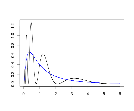
Figure 1: Two densities with the same moments

When do the moments determine the distribution?

One sufficient condition for moments uniquely determining the distribution is the Carleman condition:

\[ \sum_{i=1}^\infty m_{2i}^{-1/(2i)} = \infty. \]

You can verify that the lognormal distribution has moments which grow too quickly for this Condition to hold.