I learned about the spurious regression problem during a course at the Booth school of business. It’s well known among econometricians because it is in the classic text by Hamilton but I don’t think it’s known more widely.
A first-order measure of association between two variables \(x,y\) is their correlation. Equivalently, we can fit a univariate linear regression to the data:
\[ y = \alpha + \beta x \]
If we have \(N\) observations that are independent, given a couple mild assumptions, we get a CLT:
\[ \sqrt{N}(\hat{\beta}-\beta) \rightarrow N(0,\sigma_{y\mid x}^2/\sigma_x^2), \]
where \(\sigma_x^2 = \text{var}( x)\) and \(\sigma_{y\mid x}^2 = \text{var}( y-\alpha-\beta x)\).
We can test for association (\(\beta \not = 0\)) using a standard F-test.
The independent observation assumption is crucial. Without it, you can get very surprising and unusual behavior.
Consider observations of pairs \(x_t,y_t\), which are generated from random walks:
\[\begin{array}{ll}x_t &=& x_{t-1} + u_t, \\ y_t &=& y_{t-1} + w_t, \end{array}\]
where the errors \(u_t,w_t \sim\ N(0,1)\), are independent and \(x_0 = y_0 =0\), so both series are independent. Econometricians like to call processes like this “unit root” processes.
Theorem (Hamilton, 1994)
Suppose we have samples \(\{(x_0,y_0),\ldots,(x_T,y_T)\}\) generated as described above. Then
\[ \hat{\beta} \rightarrow \frac{ \intop_{0}^1 W_1 ( r) W_2( r) dr}{\intop_{0}^{1} W_2( r)^2 dr}, \]
where \(W_1,W_2\) are independent Brownian motions [1].
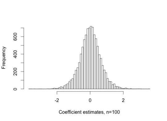
Since the two series are independent, we expect the unscaled sample correlation to converge to zero, \(\hat{\beta}\rightarrow 0\). But the theorem shows it actually converges to a random quantity. Since the limiting distribution doesn’t have a closed-form, I plot a simulation of it below. It is not that unusual for the regression coefficient to converge to a number larger than 1 in absolute value.

Figure 2: Simulation of regression coefficient distribution
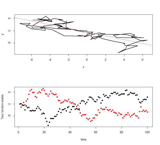
What does this mean? As the number of samples increases, the sample correlation will actually approach something nonzero (with probability one). And so in the large-\(n\) limit, the F-test will always reject the hypothesis of association. As a consequence we can easily generate a simulation of two independent variables which the F-test says are certainly dependent!

Figure 2: Two independent random walks. n=100, \(R^2\)=0.69, F-test p-value < 2.2e-16.
Cointegration
So what to do? It’s clear that an F-test is certainly the wrong thing to do to test association between two nonstationary time series, since the specificity of the test is asymptotically zero. A better approach is to test for cointegration.
Two processes are cointegrated if they are each marginally nonstationary (unit root) processes, and there exists a constant \(\gamma\) such that
\[ e_t = y_t -\gamma x_t \]
is stationary.
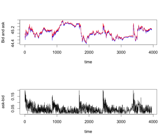
A classic example are bid/ask prices. The bid and ask are respectively the posted price for immediate sale or purchase by a market maker. These prices generally differ– their difference is called the spread. But if they differ by too large an amount, someone else will inevitably enter the market to provide liquidity, and the spread will revert back towards zero. Thus the spread
\[ s_t = p_t^a - p_t ^b \]
should be a stationary process.

Figure 3: Bid/ask prices and the bid/ask spread for a stock
To test for coinegration, there are two possibilities:
1. If the constant \(\gamma\) is known (perhaps in the bid/ask scenario we are willing to assume \(\gamma \)= 1), compute the residual series \(e_t\) and perform the Dickey-Fuller test for a unit root.
2. If the constant \(\gamma\) is unknown, estimate \(\hat{\gamma}\) with regression, and perform a special “augmented Dickey-Fuller test”.

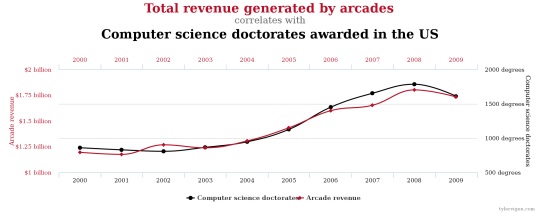
Figure 4: A spurious correlation
[1] I won’t get into what a Brownian motion is, or what the integral over a Brownian motion is. You can look at the original derivation in the source.