There is a big gap between theoretical and applied research progress for deep learning. This is a deviation from past trends in ML, such as kernel methods, which has deep roots in theory, and has enjoyed interest from both practitioners and theoreticians.

I studied statistical machine learning theory (SML) in school, and the classical thinking would suggest deep learning is actually anti-interesting. That is, there is nothing that immediately stands out about deep learning that makes it more desirable than other function approximation methods, and in fact, there are some qualities that make it problematic, such training involving high-dimensional non-convex optimization.

After school when I became a machine learning practitioner, I developed an appreciation and acknowledgement that something special was going on. Deep learning models for natural language applications was a critical component of our product at x.ai. But I was basically riding on the huge wave of institutional knowledge formed for deep learning for NLP tasks, and didn’t have good intuition about when it worked better than other approaches or why.

Generalization Error

First I’ll explain the classical statistics take on deep learning.

Suppose we have \(n\) i.i.d. realizations of the pair \((\mathbf{x_i},y_i)\), where \(\mathbf{x_i}\) is a \(D\)-dimensional real-valued vector on the unit cube \([0,1]^D\), and \(y_i\) is generated by

\[y_i = f(x_i) + \epsilon_i, \]

\(\epsilon_i\) is Gaussian noise and \(f\) is a a function \(f: [0,1]^D\rightarrow \mathbb{R}\). For some estimate \(\hat{f}\) of \(f\), we measure the its error using the integrated squared norm (with respect to the probability measure of \(x\), denoted by \(P\).)

\[ R(\hat{f},f) = \left( \intop_\mathbb{R} \mid \hat{f}(x) - f(x) \mid ^2 dP(x) \right)^{1/2} \]

To have any hope to learn \(f\) we need to make some assumptions on its structure. In the classical nonparametric literature, you put some constraints on the smoothness of \(f\), such that it belongs to a Hölder class. A function belongs to a \(\beta\)-Hölder class \(\mathcal{H}_\beta\) if it has continuous derivatives up to order \(\beta\), and the \(\beta\)-th derivative is Hölder continuous. If we let \(\beta\) be a positive integer, Hölder continuity just means that the function is bounded over it’s domain. For example, the function \(sin(1/x)\) has a second derivative which goes to infinity as \(x\) approaches 0, so it isn’t Hölder.

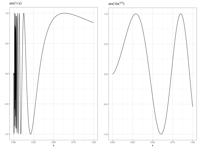
Left: A function which rapidly oscillates near 0. Right: A Hölder Function.

Now, we may ask, as the number of data samples increase, how much better should we expect an estimator to get? For a worst-case analysis, this is answered by the minimax bound, which says that for some constant \(c>0\), as the sample size grows \(n\rightarrow \infty\),

\[ \inf_{\hat{f}} \sup_{f\in H_\beta}\left\{R(\hat{f},f)\right\} > c n^{-2\beta/(2\beta + D)}. \]

This says that for any estimator \(\hat{f}\), we can find a function \(f \in \mathcal{H_{\beta}}\) that has error higher than the lower bound. There are two important implications of this.

1. The infimum is over any estimator. So the lower bound applies to any neural net estimator, any kernel estimator, etc.

2. The lower bound is pretty bad. To keep the error small, we need the number of samples to be an exponential function of the feature size \(D\). Keep in mind that for applications of deep learning, the input space is at least in the thousands. This is the statistical curse of dimensionality.

It’s also important to know that many well-known estimators can achieve this lower bound. By that I mean, the minimax bound says no estimate can have error smaller than \(O\left(n^\frac{-2\beta}{2\beta+D}\right)\), but you can also prove for many methods, including kernel methods, splines, and even neural nets, the upper-bound on the error is also \(O\left(n^\frac{-2\beta}{2\beta+D}\right)\).

Non-smooth Function Estimation

It turns out that the reason deep learning is interesting from a SML perspective is they are good at learning non-smooth functions, particularly functions that are piecewise smooth, explained by this paper:

ReLU functions can approximate step functions, and a composition of the step functions in a combination of other parts of the network can easily express smooth functions restricted to pieces. In contrast, even though the other methods have the universal approximation property, they require a larger number of parameters to approximate non-smooth structures.

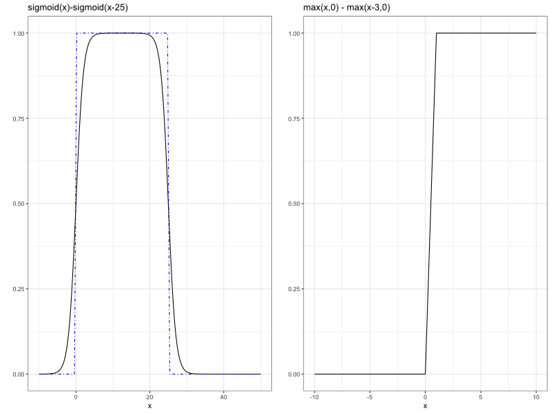
Left: Combination of sigmoid functions can approximate a step function. Right: Combination of ReLU functions can approximate a step function.

Going through the results of the paper would send us down a pretty deep hole of non-smooth function spaces etc. But here is the key part of the paper. Consider the family of linear estimators, which take the form

\[ \hat{f}_{lin}(x) = \sum \Psi_i(x,\mathbf{x_i})y_i. \]

This includes the most common nonparametric approaches, like splines, kernel estimator, and Gaussian processes, but not deep learning. Every linear estimator can not achieve the minimax lower bound if we assume the true function \(f\) is piecewise smooth, whereas deep learning achieves the optimal rate. (For that to be possible, the number of weights and layers for the neural net needs to increase with the number of samples at a particular rate described in the paper.)

The downside of this paper is it still has a curse of dimensionality – the number of samples needed to keep the error small grows exponentially with \(D\). But there are other results in the literature that suggest some methods are adaptive to the intrinsic dimension. This means that the features live on some lower dimensional manifold of dimension \(d<<D\), the estimator’s convergence only depends on \(d\) rather than \(D\). There are ways of reasoning out of the curse of dimensionality.

Pairing these ideas together, you can start to form a picture of the unreasonable effectiveness of deep learning.

The nonconvexity problem

We haven’t yet gotten to the second complaint about deep learning, which is computation. To train a deep learning model, one needs to solve a gnarly, non-convex optimization problem. Generally speaking, when you try to solve a high-dimensional non-convex problem, you are at great risk of getting stuck in the basin of attraction of a local optimum. The local optimum could be much worse than the global optimum. There are a lot of techniques for “jumping out” of the basin of attraction, but in deep learning it’s hard enough just to find a local minimum, doing further exploration is not plausible.

The computational puzzle of deep learning is: how is it that local minima are almost always good solutions?

There have been a few papers in recent years tackling this question, such as Essentially No Barriers in Neural Network Energy Landscape by Draxler et. al. The gist is that local minima tend to be pretty good for neural nets – either local minima are also global minima, or they are essentially just as good as the global minimum.

Further reading

For a collection of high-quality work to better understand deep learning, check out this course, organized by David Donoho.